
There is often a need to analyze vast amounts of spreadsheet data on many occasions. This situation makes it very difficult to gain insights quickly due to the sheer volume of datasets. For instance, you may need to infer the data on Google Sheets for making quick business decisions or come up with conclusions for your research. You may need to change cell color based on value to generate a heatmap and so on. So, what is the solution for this?
To address quick insights, Google Sheets provides the Conditional Formatting features. Here we will see whats is conditional formatting and how to change cell color in Google Sheets based on value using conditional formatting.
Content
- What is Conditional Formatting
- Change Cell Color in Google Sheets Based on Value Using Conditional Formatting
- Change Cell Color Using a Color Scale
What is Conditional Formatting
Google Sheets provides the capability to modify the formatting of any cell, based on your conditions. You can change the cell color, text format, and so on as per your criteria. Take a sample condition – “If cell D4 is empty, change its color to red.” Let us look into the various components involved in this condition.
- Range – This component defines the cell or range of cells you want the criteria to be applied. (In the above example, it is cell D4.)
- Cause – The trigger event that causes the color change/formatting. (Here, the cell D4 being empty causes the trigger.)
- Outcome – Once the cause trigger occurs, what change should happen? This change defines the outcome. (The color of cell D4 changes to red is the outcome.)
Change Cell Color in Google Sheets Based on Value Using Conditional Formatting
For this guide to change cell color based on value in Google Sheets, consider a sample dataset of students’ names (Column A), their marks in a test (Column B), and their attendance in percentage (Column C). The criterion we are about to define is to change cell color to green if a student passes the test (Marks greater than 50). Also, change the cell color to red if a student fails the test (Marks less or equal to 50). Let’s see the steps involved to execute this easily.


- In the Google Sheets spreadsheet, select the cell/range of cells whose color you wish to change on the spreadsheet.
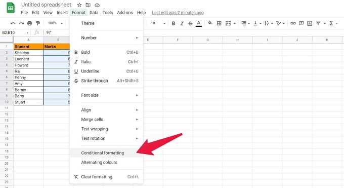
- Click on the “Format” tab and choose “Conditional Formatting.”

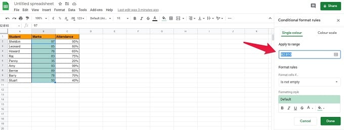
- Within the “Apply to range” section, you can see the range of cells (B2:B10) on which the color change is to be applied. (There is also the option of manually entering the cell/cell range in case of many cells.)

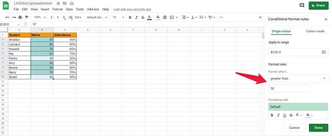
- Next, click on the dropdown under the “Format rules” section. Here you can choose the trigger of the condition. From the different options available, we have selected the “Greater than” condition and value as 50. (Other in-built / custom conditions can also be defined here based on the need.)

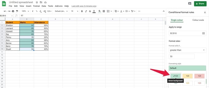
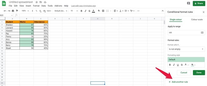
- Select the formatting style needed once the trigger condition is satisfied. By default, Google Sheets will change the cell color to green.

These steps (1-5) will ensure that all students who have passed the test will have their marks highlighted in green.
- To change the cell color of failed students, click on “Add another rule.”

- In the “Apply to range” section, enter the cell range (B2:B10 in this case) on which the color change is to be applied.
- As we did earlier, click on the dropdown under the “Format rules” section. From the different options available, select the “Less than or equal to” condition and value as 50.

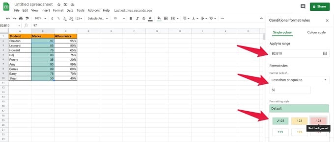
- In the “Formatting style” section, select the color as “Red.” (Users have the flexibility to choose different text formatting options and custom colors apart from the basic ones shown.).
- Click on “Done.”

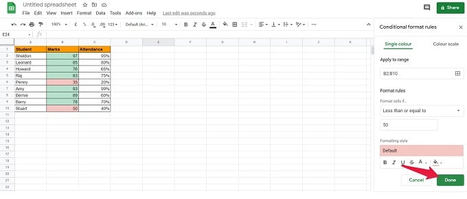
With these steps, we have successfully changed cell color based on the value in Google Sheets. We have achieved the desired outcome of the defined criteria.
Similarly, we can change the cell colors based on text values, dates, and other custom conditions. These capabilities make Google Sheets a powerful formatting tool.
Change Cell Color Using a Color Scale
The Color Scale option allows you to format cell colors within a spectrum of colors. This functionality can help check if specific goals are met by various employees of an organization, team members, students, etc. Next, let’s discuss the steps to change cell colors based on value using the color scale. We are using the Column C of the earlier dataset (Attendance %) to demonstrate this feature.
- Click on the “Format” tab and select “Conditional Formatting.” Click on “Color Scale.”
- Within the “Apply to range” section, you can set the range of cells (C2:C10) on which the color changes are to be applied.

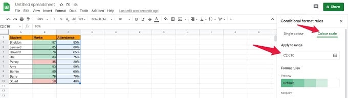
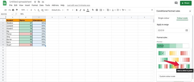
- Next, click on the color spectrum below “Preview” under the “Format rules” section.
- Choose the set of colors you wish to apply to the column based on a range of values. We have selected red for low values of attendance, white for medium values, and green for high values in this example.

- Once the colors and intervals are defined, click on the “Done” button.

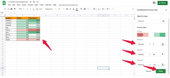
There you have it! The attendance percentage of students being categorized based on different intervals using a color scale.
In this guide, we have covered a sample scenario of changing cell color based on the value in Google Sheets. We can apply this feature of Conditional Formatting to a wide range of academic and business scenarios. Google Sheets is, therefore, a comprehensive tool for gaining quick insights from your critical datasets.


