
Are you someone who regularly uses formulas on Google Sheets? There’s good news for you. Recently, Googled introduced a new Formula Corrections feature that provides suggestions to help you to fix wrong formulas or do improvisations.
Let’s see how to use the Formula Corrections on Google Sheets to fix wrong formulas.
How to Enable Formula Corrections on Google Sheets
You don’t need to do anything as the formula corrections feature is enabled by default. According to Google Support Page, this new feature will help you improve and troubleshoot complex formulas.
For example, this feature can detect errors while using the VLOOKUP function, missing cells in range input, and much more. This feature will be available to all users who use Google Sheets.
Related: How to Create Real-time Crypto Portfolio Tracker with Google Sheets
Fix Formula Errors Using Formula Corrections on Google Sheets
You will see a suggestion box if the Google Sheets detects an error or improvement, whether you are entering a simple or complex formula. You can either accept the suggestion or decline it. Let’s look at how Formula Corrections work on Google Sheets with a couple of examples.

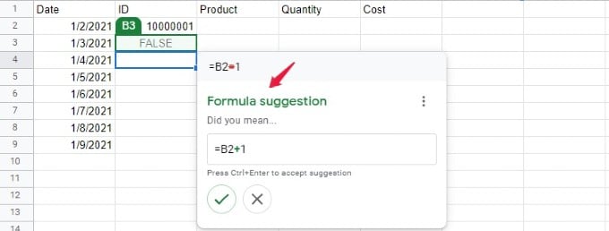
Here’s a simple example. In the above image, you can see that instead of typing ‘+’ to add 1 to cell B2, you might have wrongly typed it as ‘=.’ Sheets has detected that and displays the formula suggestion. You can press CTRL + Enter or click the ‘Tick‘ icon to accept the suggestion and fix the error. Or you can click the ‘X‘ icon to ignore the suggestion.
Now, let’s take a complex example of using the VLOOKUP function.

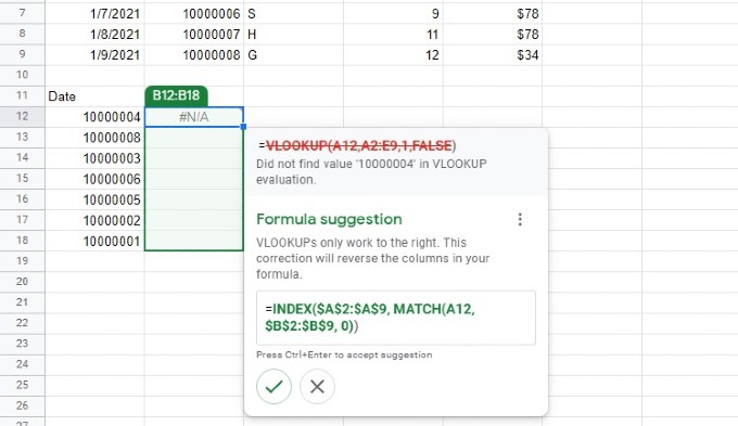
In the above example, you are trying to search data using the VLOOKUP function. And in the suggestion box, you can see that the correction suggests that VLOOKUPS only work to the right and suggests using a combination of INDEX and MATCH to reverse the columns in your formula. By accepting the suggestion, the formula will correct itself and include possible cells/rows/columns for the function.
Related: How to Quickly Highlight Duplicates in Google Sheets
How to Disable Formula Corrections on Google Sheets
Are you very confident in working with formulas, and do you find the formula suggestions quite annoying at times? You can easily disable the formula corrections feature with a single click.
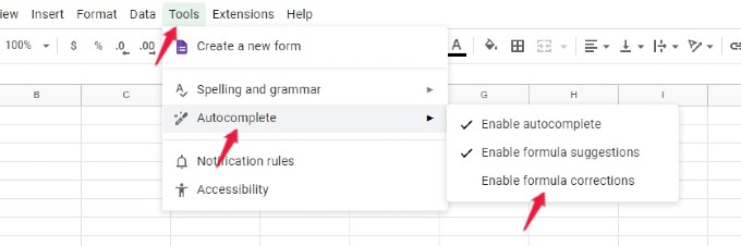
Open Google Sheets on any browser on your computer. Then, click Tools in the top toolbar. From the list of options displayed, move your mouse over Autocomplete and then click Enable formula corrections.

You don’t see a tick mark on that setting? That’s it. Now, you will not see any formula corrections anymore.
We have tried the Google Sheets formula corrections with a couple of examples. However, you can try using the feature for different formulas and see how it helps.


