If you are a Google Sheet user, you would have probably noticed that when you scroll down the top header rows disappear. While dealing with large-sized datasets, the chances are that you may forget each column’s names and you are unable to view them while scrolling. To overcome this issue, we will talk about the “Freeze Rows” in Google Sheets. Upon enabling this feature, Google Sheets will lock the particular row(s). These rows will then be visible even while you scroll down through your spreadsheet.
There are multiple ways by which you can free rows in Google Sheets at top. Here are they.
Freeze Rows in Google Sheets Using Shortcut
You can simply freeze rows in Google Sheets with a few clicks using your mouse. You just need to select the rows you want to freeze and follow the steps below.
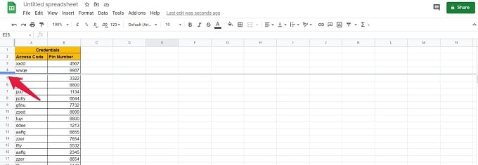
- Place your mouse cursor to the top left corner of the spreadsheet. Place it above the horizontal part of the grey border as shown.

- Once the mouse cursor transforms into a hand-like icon, click and drag it down to Row 1 if you want to Freeze only Row 1. Drag it till Row 2 if both Row 1 and Row 2 are to be frozen. Similarly, you can Freeze multiple rows in Google Sheets as per need.

There you have it. First, two rows are now Frozen, allowing an easy view of column heads during scrolling down.
Freeze/Lock Rows Using Google Sheets Menu Option
Instead of dragging and dropping to lock rows in Google Sheets, you can use the Freeze function from the Google Sheets menu.
- Go to the top menu in Google Sheets. Then, click on the “View” tab. And, select the “Freeze” option.
- From the drop-down, select the option to Freeze any number of rows. If you only want to Freeze Row 1, select “1 row“. If you wish both Row 1 and Row 2 to be maintained in a Frozen state, select the “2 rows” option from the drop-down.

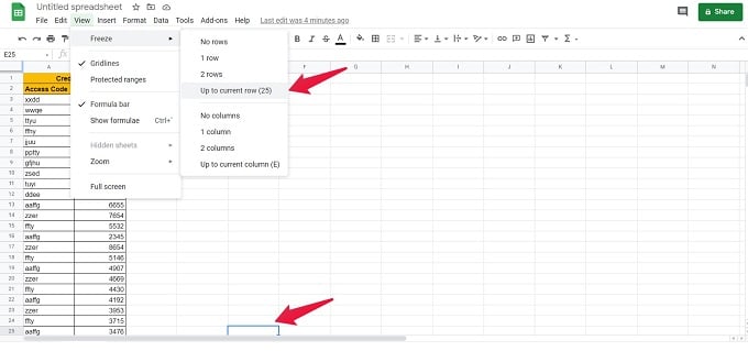
- Similarly, if you want to Freeze the first 25 rows, select a cell in Row 25. Again, Go to the top menu in Google Sheets. Click on the “View” tab. Select the “Freeze-*” option.
- From the drop-down options, you will notice “Up to current row(25)” given. Click on that option. This action will Freeze the first 25 rows successfully.

As you can see, the Google Sheets lock row functionality is neat and straightforward to execute.
Unfreeze Rows in Google Sheets Using Shortcut
What if you wish to Unfreeze the rows you did freeze to the top at a later point in time? What is Frozen can be Unfrozen in Google Sheets. Let’s see how to unfreeze locked rows in Google Sheets using mouse shortcut.
- Place your mouse cursor below the Frozen row of the spreadsheet as shown.

- Once the mouse cursor transforms into a hand-like icon, click and drag it to the row above if you want to that row alone. For instance, if Row 4 is frozen and you wish to unfreeze only that row, drag the hand-like icon up to Row 3. This action will Unfreeze Row 4.
- If you want to Unfreeze all rows, drag the hand-like icon up to the spreadsheet’s top left corner. This action will Unfreeze all rows.
Unfreeze Rows Using Google Sheets Menu Option
Like you can freeze rows in Google Sheets, the menu also has the option to unfreeze single row or multiple rows in the spreadsheet.
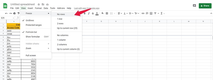
- Go to the top menu in Google Sheets. Then, click on the “View” tab. And, select the “Freeze” option.
- From the drop-down, select the option “No rows.” This step will Unfreeze all rows that were previously in the “Freeze” state.

Unfreezing of Rows is complete, and it is an effortless feature that makes the Google Sheets freeze row procedure easily reversible on demand.
As discussed here, you can freeze multiple rows in Google Sheets in simple and quick ways. This feature makes viewing large datasets in your spreadsheet rather convenient. It also lets you Freeze and Unfreeze the Columns of spreadsheet data. This aspect makes scrolling and analyzing data horizontally less complicated.
