Conditional Formatting on Google Sheets: Everything You Need to Know

These days, a lot of people prefer Google Sheets to Microsoft Excel for many reasons like zero cost, multi-user access, cloud storage, and most importantly you can access spreadsheets on the go from your smartphone. In addition to being the #1 user-friendly spreadsheet tool, Google Sheets also offer a cool feature called Conditional Formatting that helps users to quickly analyze complex or lengthy sheets.

In this post, let’s take a look at some of the ways to use conditional formatting on Google Sheets.

What is Conditional Formatting

It is a feature that allows you to modify/change the aspect of a cell, based on a single or set of rules. You can change several aspects of a cell, like its background color, text type (Bold/Italic/Underline). Regarding rules, you can either use the existing ones available on Google Sheets or you can create your own rules as well.

Based on your requirements, you can apply conditional formatting to a single cell, group of cells or to an entire row/column.

Related: How to View and Remove Authorized Apps From Google Account

Rules – What Does it Mean

Before thinking of using conditional formatting, first, you need to understand the structure of rules. Every rule consists of the following three elements:

• Range – Defines the scope of the rule. For example, let’s say that you would like to format cells from B2 to B22, based on a condition. In this case, the range is set to 20 cells.
• Condition – Defines trigger events. In the example above, let’s assume that you need to format the cells if its value is greater than 10.
• Style – Defines the style of the cell. Like, change the background color of cells to blue.

So? The rule for the above example is something like this: If any value of the cell from B2:B22 is greater than 10, then change its background color to blue.

How to Use Conditional Formatting on Google Sheets

Now, let’s see in detail the various types of conditional formatting that can be used on a cell, row or column in Google Sheet.

Conditional Formatting with Numbers

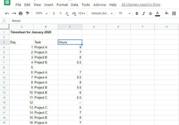
Let’s imagine that you are evaluating the monthly timesheet of someone in your company. And, you need to find out whether he/she has logged in for at least 7 hours on all working days for that month. The timesheet looks similar to the one below:

Let’s see how to use conditional formatting for this scenario.

1. Open the timesheet file and navigate to Format->Conditional formatting.
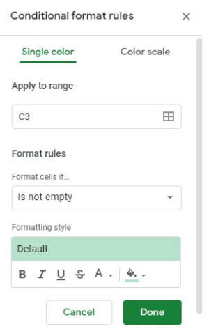
2. Here, you will see a new window titled Conditional format rules on the right side of your screen. By default, Single color tab will be selected:
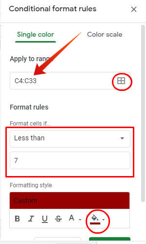
3. In the drop-down box titled Apply to range,  click Table icon, select the range as C4:C33 and click OK.
4. Under Format rules drop-down box, select Less than.
5. Next, enter 7 in the box titled Value or formula.
6. Then, under Formatting style, set Fill Color to your desired color. Instead of changing the background color of the cell, you can modify text color or set other formatting options like Bold, Italic, Underline and Strikethrough.
7. Finally, click Done.

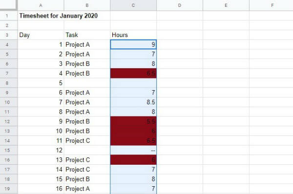
Now, if you observe the above image, days for which working hours are less than 7 are highlighted (Column C).

For conditional formatting with numbers, you can use any of the conditions listed below:

• Greater than
• Greater than or equal to
• Less than
• Less than or equal to
• Is equal to
• Is not equal to
• Is between
• Is not between

Conditional Formatting with Text

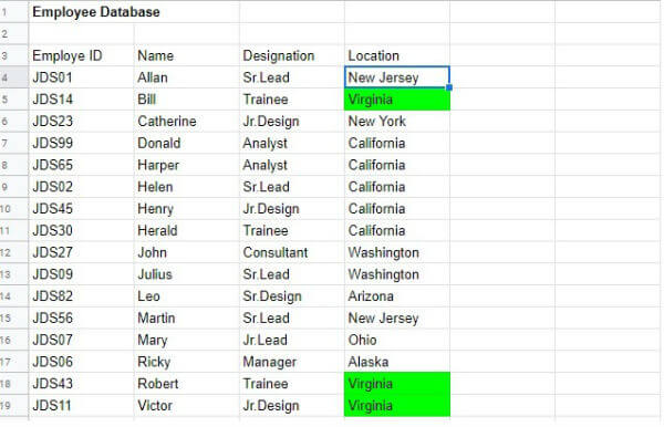
Let’s say your employee database sheet has hundreds of entries and you wish to highlight employees residing in a particular location (eg. Virginia). You can easily do that by using Conditional Formatting with Text.

1. Open the employee database file and navigate to Format->Conditional formatting and look for the window titled Conditional Formatting on the right side of your screen.
2. In the drop-down box titled Apply to range,  click Table icon, select the range as D4:D104 and click OK.
3. Under Format rules drop-down box, select Text contains and type Virginia in the box provided below.
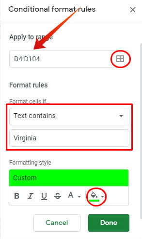
4. Then, under Formatting style, you can change either the text/background color of cell or other options like Bold, Italic, Underline or Strikethrough. In this example, Fill Color is set to Green.
5. Click Done. Now, all employees who are located in Virginia are highlighted as given below:

Other available options for conditional formatting with text are:

• Text starts with
• Text ends with
• Text is exactly
• Text contains
• Text does not contain

Also read: What is Sharing Violation Error in Excel and How to Solve It

Conditional Formatting with Color Scale

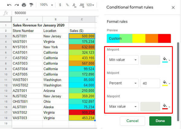
Formatting with color scale will come in handy if you need to analyze data for levels like minimum, maximum and average. For example, a business seller can use this formula to quickly analyze the sales revenue in different locations. Let’s see how to do that.

1. Open the file and navigate to Conditional Formatting window.
2. Next, click tab titled Color scale.
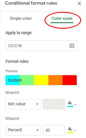
3. Then, select the range of cells for which you need to apply the rules.
4. Here, you will see three drop-down boxes titled: Minpoint, Midpoint, Maxpoint. Based on your requirement you can select either Number, Percent or Percentile.
5. In case you would like to set a specific value for Midpoint, Minpoint or Maxpoint, you can do that by entering the numbers in the corresponding boxes. In this example, we have selected 40 Percent for Midpoint.
6. Next, select your desired colors for all the three checkpoints, if you don’t like the default color settings.
7. Finally, click Done.

More Conditional Formatting Options

Apart from number, text, color range, there are two more options available on the conditional formatting window:

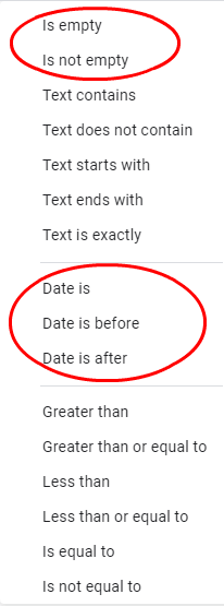
Is Empty/Is Not Empty

This is the simplest option in conditional formatting. If you want to highlight only a group of empty or non-empty cells, then you can use this feature. To locate this option, just click the drop-down box titled Format Cells in Conditional Formatting window.

Date

This formula will come in handy especially if you would like to compare your data over a specific range of dates or a single date by clicking the drop-down box titled Format cells if:

• Date is
• Date is before
• Date is after

Once you select any of the above date options, you will see another drop-down box as shown below:

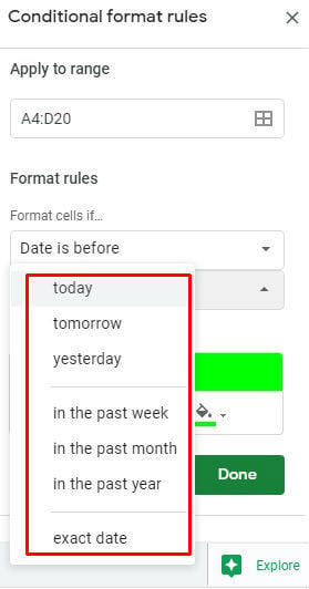
Based on your requirement, you can select any of the options to create the date based rule.

Related: How to Create Google Forms Online for your Business?

How to Use Conditional Formatting Over an Entire Row in Google Sheet (Custom Formula)

So far, in all the examples mentioned above, single or multiple cells in a column were highlighted. But, what if you need to do conditional formatting of a row in Google Sheet instead of a cell?. Thanks to the Custom Formula option, you can easily do that.

Now, let’s consider the example mentioned in the section Conditional Formatting with Text. Instead of marking only the cell that contains text “Virginia”, let’s try to highlight the entire row.

1. Navigate to Conditional Formatting window after opening your file.
2. Then, you have to select the entire data set for range, since we need to apply conditional formatting over an entire now. In this example, we have selected range as A4:D20.
3. Next, select the option Custom formula is, in the drop-down box titled Format rules.
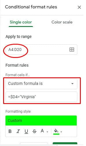
4. Here, you need to enter the formula as =$D4="Virginia" on the box provided below. Now, let’s try to understand how this custom formula works.= : Any custom formula should begin with this character.
   D4 : indicates your sample data. i.e D4 is the first cell of column D whose data is analyzed.
   =”Virginia”: defines the condition. Since we need to highlight rows of employees located in Virginia, = is used. In case you would like to mark employees who are not located in Virginia, you can use <>”Virginia”. Likewise, you can create conditions that involve numbers using symbols like >, <, >=, <=, etc.
5. Finally, click Done.

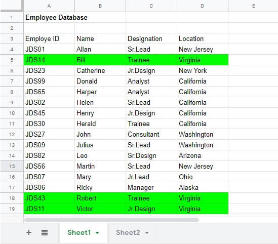
Did you see? Now, the entire row is highlighted instead of a single cell for the employees located in Virginia.

Well, we have explained just simple examples of using conditional formatting in Google sheets. Depending on your need, you can create any custom formula you like to get a quick analysis of a huge amount of data.