Do you need to analyze a spreadsheet with a huge amount of data? Well, it will be a great challenge especially if you are not a big fan of numbers. To make things easier, you can make use of the Filter function available in Google Sheets to view the data only you want to see.
In this post, let’s see how to create and use a filter in Google Sheets.
Create a New Filter in Google Sheets
Though you can make use of filters to analyze any massive spreadsheet, let’s go with a simple example. Let’s say you are analyzing a spreadsheet that contains the details of a person’s workout with fields like distance, duration, pace, timestamp, etc.
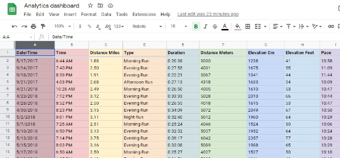
And, you need to find out the days on which the person has covered the minimum distance of the workout plan. (eg. 3 miles )
Now, let’s see how to create a filter to do this.
Open the Google Spreadsheet file on your computer.
Select the columns A(Date), B(Time), and C(Distance Miles).
There are two options to create a filter. After selecting the columns, click the menu Data and select Create a filter from the list of options.
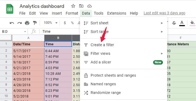
Or you can click the Filter button in the toolbar.

Now, you will see a filter icon in the top cell of every column you had selected.

Related: How to Hide Columns in Google Sheets
Filter By Condition
In our example, we want to see the days on which the person has covered a distance of at least 3 miles. Since we are interested in viewing only the data that satisfies certain criteria, we have to use Filter by condition.
Click the Filter icon on column C and then click Filter by condition.
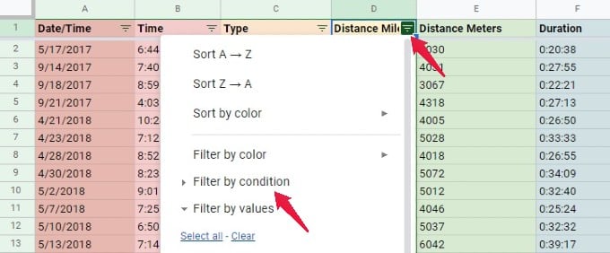
Here, if you click on the arrow, you will see many conditions listed like the one below.
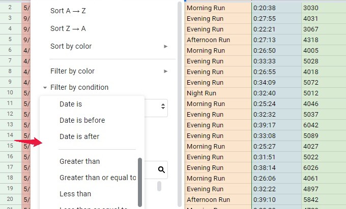
Go ahead and select the option Greater or equal to and type the number 3 in the provided box.
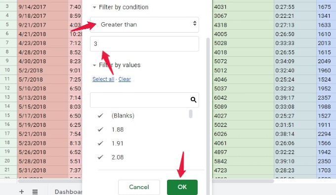
Finally, click the OK button.
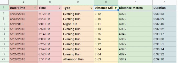
Now, you will see the workout data only for those days during which the person covered the minimum distance.
Related: How to Wrap Text in Google Sheets Cells to Show Full Text in Google Sheets
Filter By Value
In our example, let’s say you want to check out the days on which the person has completed the workout in the morning. In the sheet, you can see that column D(Type) has either one of the values: Morning Run, Afternoon Run, Evening Run, and Night Run. Let’s see how to use the Filter by Value option.
Select columns A to D and create a filter.
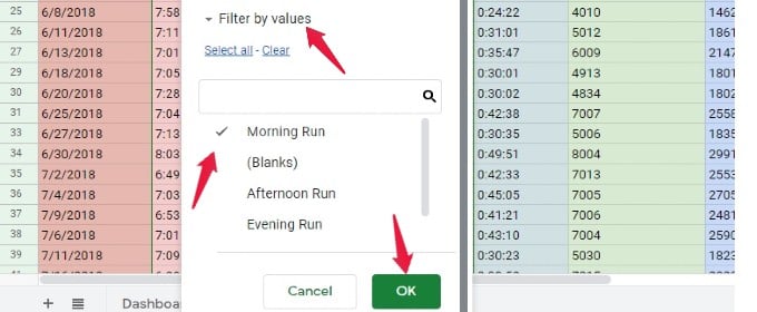
Then, click the Filter icon on Column D and select the option Filter by values.
Here, you can see a tick mark for all the values. Since we are interested only in the morning run, deselect all other values and click the OK button.
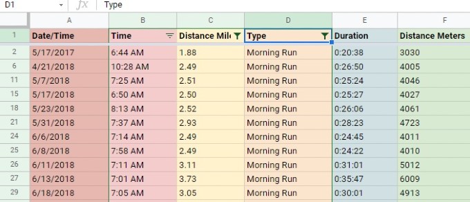
Now, the sheet will show the data only for the morning run.
Save Filter View in Google Sheets
Sometimes, you might need to use more than one filter in a sheet for analysis. In such scenarios, it will be better to save the filter view and use it whenever needed.
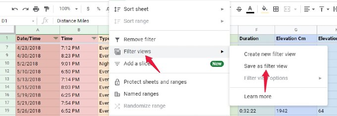
Let’s say you are viewing the filtered data. To save this view, click Data.
Then click Filter views > Save as filter view.
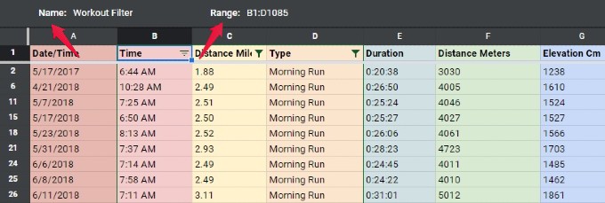
Here, you will see a black border around the cells with two fields Name and Range. In the Name field, enter a name for the filter view. The range indicates the cells that will be used for filtering the data. Make sure you have selected all the cells/columns that are required.
That’s it. Now, the filter view has been saved successfully and you can use it whenever you need.
To reuse the saved view, click Data > Filter views. You can see the list of all filter views you had created. If you click on a particular view, then that filtered view will be applied to the current Google sheet you had opened.

Related: How to Change Cell Color in Google Sheets Based on Value
If you share a Google Sheet with others, they will get access to the filters as well. This will come in handy when you are analyzing the sheet with a group of people.
