
Duplicate data in a large spreadsheet is a waste of your time and causes confusion. If you have an excel file, you can easily find and highlight duplicates in Google Sheets by analyzing your data. It only takes a couple of formulae to solve the duplicate entries issue on your spreadsheet.
Let us see how to find and eliminate duplicate data in Google Sheets from your computer.
Highlight Duplicates in Google Sheets on a Single Column
When multiple people have access to a Google Sheet and anyone can edit the data, then there is a higher probability of duplicate entries. Fortunately, you can use the Conditional Formatting feature of Google Sheets to quickly highlight duplicates. Let’s see how to do that.
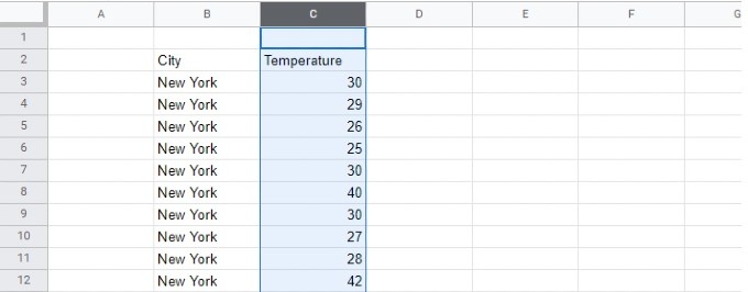
Open the Google Sheet file on your computer using any browser. Then, select the column in which you need to find out the duplicate entries. (eg. Column C)
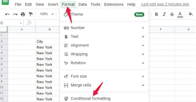
Click the Format menu on the top and then select Conditional Formatting from the list of options displayed.
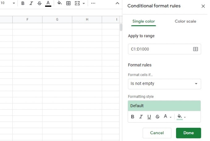
On the right side, you will see a new window titled Conditional format rules.
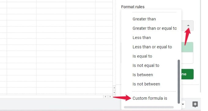
Click the drop-down box below Format rules and select Custom formula is.
Type the below formula on the box provided
=countif(C1:C,C1)>1
Then, under Formatting style, click the Fill Color icon and select the color you wish to highlight the duplicates.
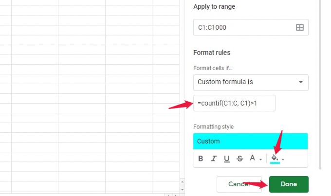
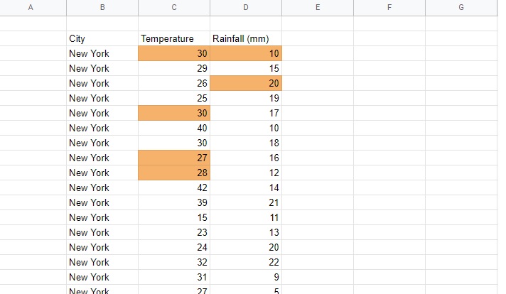
Finally, tap Done to highlight the duplicates in the color you had selected.
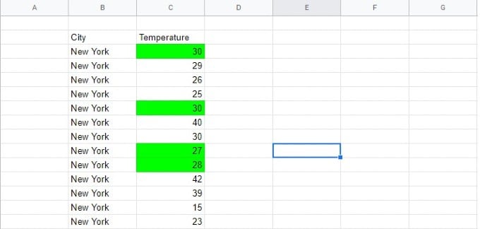
The highlighted cells are duplicated in your spreadsheet. That means the same data is repeated more than once in the same column.
Related: How to Create and Use Filter in Google Sheets
Highlight Duplicates in Selected Cells on Google Sheets
Let’s say you need to find duplicates only for a selected range of cells instead of the entire column. To do that, enter the data range (eg. C4: C20) in the box below the “Apply to range.”
Then, you need to enter the below formula:
=countif(C4:C,C4)>1
where C4 indicates the first cell of the data range you had selected.
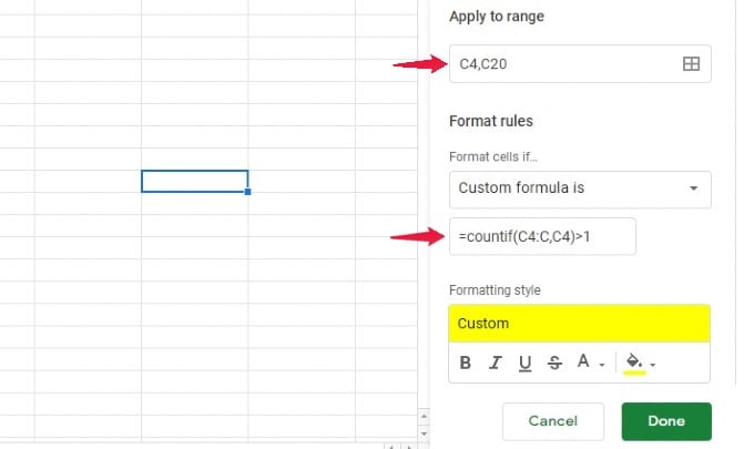
When you click “Done“, you will see the duplicate data highlighted in the cells you selected only.
Related: How to Hide Columns in Google Sheets
Highlight Duplicates in Multiple Columns on Google Sheets
Do you need to highlight duplicates in two columns or more? You can easily do that by selecting multiple columns at a time and applying the formula. Let’s see how to do that.
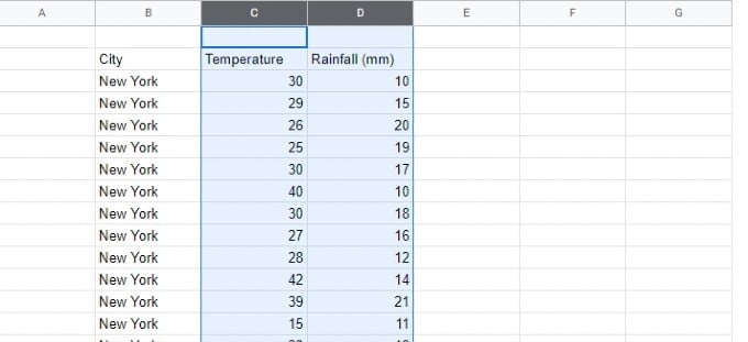
Open the Google Sheets file and select all the columns (eg: Columns C and D) for which you need to find duplicates.
Click the Format menu on the top and then select Conditional Formatting from the list of options displayed.
On the right side, you will see a new window titled Conditional format rules. Click the drop-down box below Format rules and select Custom formula is.
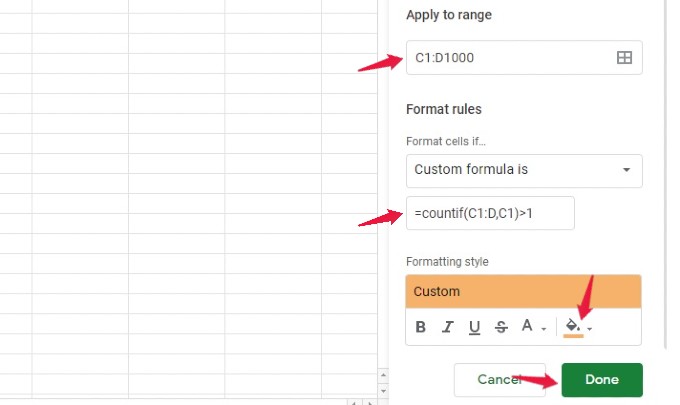
Type the below formula on the box provided
=countif(C1:D,C1)>1
Then, under Formatting style, click the Fill Color icon and select the color you wish to highlight the duplicates.
Finally, tap Done to highlight the duplicates in the color you had selected.
In case you wish to find duplicates for many columns like from B to F, then the formula will be
=countif(B1:F,B1)>1
Do remember that you can highlight duplicates in multiple columns at once. However, you cannot have a separate color for every column. If you want to have different colors for different columns, then you need to follow the single-column method and repeat that for all columns.
Related: How to Wrap Text in Google Sheets Cells to Show Full Text in Google Sheets
How to Remove Duplicates in Google Sheets
So far, we have seen how to quickly highlight duplicates in multiple rows and columns of a Google Sheet. After finding the duplicate entries, let’s say you want to get rid of those rows that contain them. Let’s see how to do that.
In the Google Sheet, select the data range from which you need to delete the duplicates.
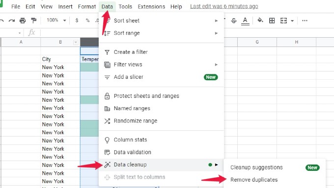
Then, click the Data menu located on the top. From the list of options, move your mouse over the option Data cleanup.
Here, you will see another small pop-up menu. Go ahead and select Remove duplicates.
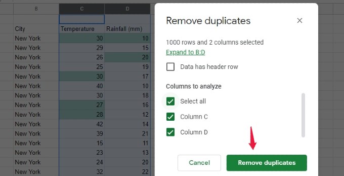
Then, you will see a pop-up menu that displays the details of the data range that is selected. (If your data has a header row, then select Data has header row option)
Finally, click Remove Duplicates.
That’s it. Now, the duplicate entries in the rows have been deleted successfully and you will see a success message for the same.
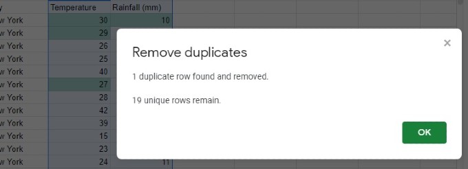
When selecting multiple columns, a row will be considered as duplicate only if all the values in that row matches with another row.
Related: How to Use Formula Corrections on Google Sheets: Fix Formula Errors Automatically
Well, it is not necessary that you need to use this feature only for highlighting duplicates. You can also use this just if you need to highlight the number of occurrences of a particular data.