
Google Sheets Application is an excellent alternative to Microsoft Excel to work on spreadsheets on the fly. There is the flexibility to use Google Sheets from a web browser. The need to install the same locally on your PC is eliminated. If your work demands you to handle many spreadsheets, there may be a need to “Transpose” your data often. Transpose is the mathematical operation of converting Rows to Columns and vice-versa. (A “Row” is a set of values/numbers along a horizontal line. A “Column is a set of values/numbers arranged along the same vertical line.)
In this article, we will discuss a couple of easy ways to execute google sheets transpose, i.e., convert rows to columns and the other way around.
Convert Rows to Columns in Sheets Using Paste Special
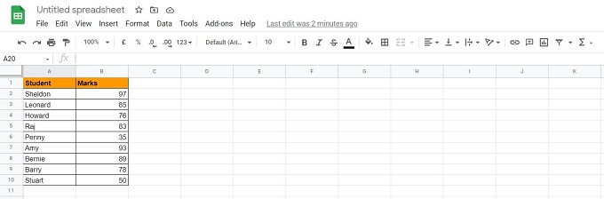
Before you move ahead with transposing our data, you need to key in the data itself on your Sheet. Open a new Google Sheet on your browser. Input the required data. Consider an example where you wish to transpose a couple of columns with the name of a few students and the marks they scored in a test. This is shown below. Column A depicts the Student names and Column B gives their respective Marks scored in a test.
Transposing the above data means that the name of the students would appear in a single row and their marks in the row below the names. Transposing the above data means that the students’ names would appear in a single row and their marks in the row below the names.
- Select all the cells with your required data. Click Ctrl+C to copy the data.
- Click on the target cell. This cell would be from where you want your transposed data to get populated on the Google Sheet. In this case, we have selected cell D3 for pasting the target transposed data.
- Once your target cell is selected, perform a right-click.
- Select the “Paste Special” option. From the drop-down, click on “Paste Transponsed.”
- And there you have it! The columns are converted into rows. It is as easy as that. Row 3 has the data held previously by Column A. Row 4 consists of the data that was in Column B.
- To perform the reverse conversion, you need to follow the above steps. In this case, the original data to be arranged in row format. You will get the transposed data arranged as columns.
The advantage of using the Paste Special Method is that it copies the formulas, values, and formatting along with the values. Having understood the Google Sheets’ switching of rows and columns using the Paste Special Method, let’s move ahead to the next one.
Convert Rows to Columns in Google Sheets Using Transpose Function
One of the primary reasons why Google Sheet is gaining widespread popularity is the presence of some useful built-in functions. This feature makes the lives of students and professionals very easy. The work gets done with minimal effort.
The “Transpose” function is one of these built-in functions. The Transpose is designed to convert your row data into columns automatically and vice-versa.
- Once you have your dataset keyed in, select a target cell.
- To input the Transpose function, type “=Transpose(“ followed by selecting all the cells containing your data. Doing so will show the range of cells within your Transpose function. We have chosen cell D3 to apply the Transpose function. The data in Columns A and B till Row 10 is selected.
- Hit Enter. There you have it! Your columns have been converted into rows.
Google Sheets is smart enough to automatically identifies the number of rows and columns and populates the target cell with the appropriate cell value. Data from Column A is populated in Row 3. Data from Column B is now placed in Row 4.
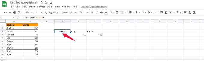
Please ensure that there is a required number of empty target cells to accommodate the transposed data. If there are any cells with particular number/text or even a Space character, Google Sheets will give you a Reference Error. (Denoted by #REF!) The entire dataset will disappear, and the “#REF!” can be seen in the top-left cell of your set of cells.
In the scenario shown below, an attempt was made to apply the Transpose function in cell E3. As E3 already contained data from the previous Transpose operation, Google Sheet notifies a Reference Error in cell D3.
There are a couple of differences between Method 1 and Method 2:
- Using the Transpose function only performs the data conversion from Row to Column-wise arrangement. The cell formatting is not replicated in the target cells. This situation was evident in Paste Special Method.
- Transpose function is dynamic in nature. Any changes made in the cells consisting of the original data will be reflected in the target transposed cell.
This scenario is not the case with Paste Special Method. Any changes made in the original cell will require the same modification to be created manually in the target cell.
We hope you found value in the two methods in google sheets to convert rows into columns. These are pretty simple to execute and require minimal technical skillset dependency.