How to Make Pie Chart Using Google Sheets: Quickest Ways to Create and Edit Pie Charts

Graphs and Charts help us to quickly understand any kind of data. Though there are a lot of ways like Bar charts, Line graphs, and Mekko charts to visually represent data, Pie Chart is the simplest one. You can create pie charts quickly with Google Sheets from your computer.

In this post, let’s see how to create and customize a Pie Chart using Google Sheets.

How to Create Pie Chart in Google Sheets

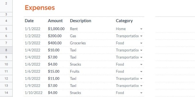
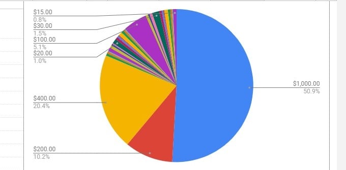
Let’s take the simple example of your personal monthly expenses or your family’s. In case, you want to quickly find out how you are spending the money, you can easily do that by using the Pie chart.

On any browser on your computer, go to sheets.google.com and open the Google Spreadsheet document.

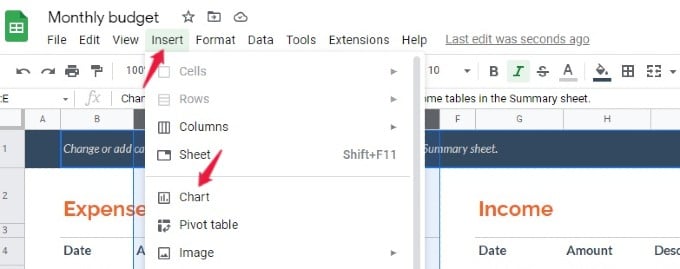
Select all the cells that contain the data to plot the pie chart. Then, click the Insert menu at the top and click Chart from the list of options shown.

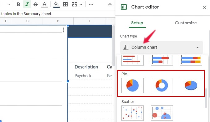
After you click Chart, the graphical representation of the selected data will be shown. If it is not a Pie chart, then double-click the chart. Now, you will see the Chart editor window on the right. In that, click the tab Setup. Then, click the drop-down box Chart type and select any of the Pie chart types.

Now, you will see the Pie chart for the data you had selected earlier.

In the Setup tab, you will see multiple options to edit the chart.

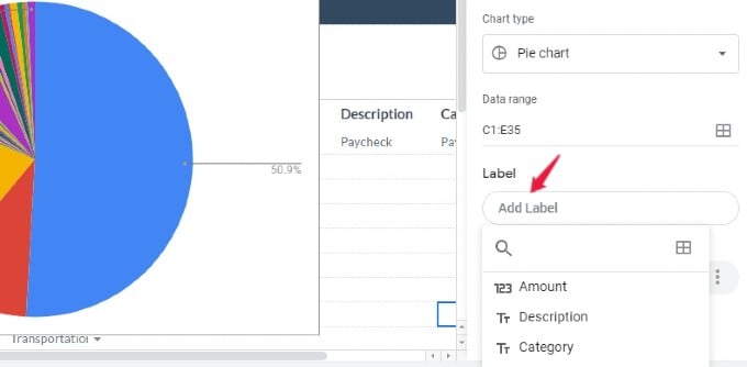
Label: This field defines the label for the Pie slices in the chart. In this example sheet, there are three columns Amount, Description, and Category. Based on your selection, the labels will be displayed. For example, if you select Amount, then the Pie slices will be labeled using the amount.

Data range: If you think you had left out some cells or need to add new data, then you can click the table icon. Then, a new window titled “Select a data range” will be displayed where you can edit or add new data set.

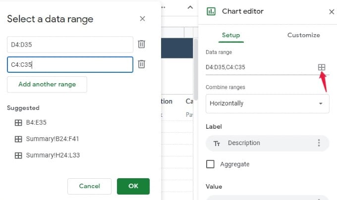
Also, you can use rows as headers, columns as labels, and switch rows/columns using the below options.

Related: 10 Best Budgeting Apps for Android and iPhone

How to Edit/Customize Pie Chart in Google Sheets

Google Sheets offers a lot of options to customize the style and appearance of the Pie chart. The settings are categorized under five sections: Chart style, Pie chart, Pie slice, Chart & axis titles, Legend. Let’s explore them one by one.

Double click the Pie chart to view the Chart editor. Then, select Customize tab. From there, you can make numerous changes to the pie chart and make it look better.

Change Google Sheets Pie Chart Title

Do you wish to create a unique title for your Pie chart? You can do that by selecting Chart title from the drop-down box in Customize tab.

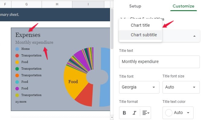
You can then enter the title in the box provided. You can also create a subtitle for the chart by selecting Chart subtitle. Plus, you can modify the font type, size, color, format, and alignment for the title and subtitle.

Related: How to Quickly Create a Drop-Down List in Google Sheets

Edit Legends in Google Sheets Pie Chart

The colored labels you see along with the piece chart are called legends. If you want to edit the position of these legend labels in the pie chart on Google Sheets, you can do that.

After double-clicking your pie chart, go to the Customize tab. From there, click to expand the “Legend” option.

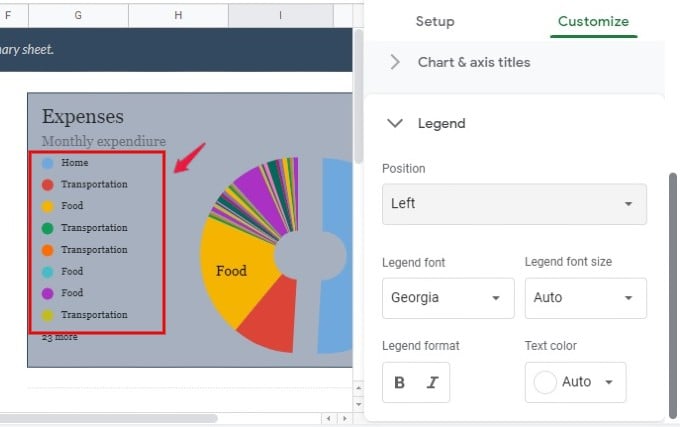
In this section, you can change the position of the legends by selecting Top, Bottom, Left, and Right from the drop-down box Position. Also, you can change the font type, color, size, and format as well.

Show Labels in Google Sheets Pie Chart

Do you want to show text labels on top of the pie chart you just created in Google Sheets? It is always good to add labels to a pie chart to understand things better.

When you double-click the pie chart and go to the Setup option, you will see the labels menu there. If this field is set to None, then there will not be any text shown on the Pie slice. If it is set to Label, then the label will be displayed on the Pie slices. You can also set this field to Value/Percentage.

You can also change the font color, size, and format for the label here.

How to Create 3D Pie Chart in Google Sheets

From the Chart Style option in Customize tab, you can change the background color and border for the Pie chart in the Chart style. Also, you can change the font type for the text in the Pie chart. From the same, you can also make 3D pie chart in Google Sheets.

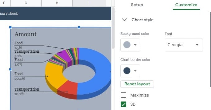
If the checkbox 3D is selected, the chart will be displayed in the 3D view. If the checkbox Maximize is selected, then the labels will be removed and the Pie chart will be shown in a much bigger size.

Related: How to Quickly Highlight Duplicates in Google Sheets

How to Create a Donut Chart in Google Sheets

You can put a hole in the center of the pie chart and make it a donut chart on Google Sheets. For that, double-click the chart and go to the Customize tab. From there, click and expand the Pie Chart menu.

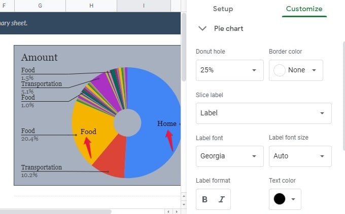
In this section, you can adjust the size of the donut hole. If the value is set to 0%, there will not be any holes in the chart. If you set the value to 25%, 50%, or 75%, then the donut hole will vary based on your selection.

Separate Pie Chart Slices in Google Sheets

If you want an easy-to-read format for your pie chart, you can separate the pie slices and keep them apart. To create separate pie slices in Google Sheets, double click the created pie chart or donut chart and go to the Customize tab from the right. From there, select the “Pie Slice” menu to see the available options.

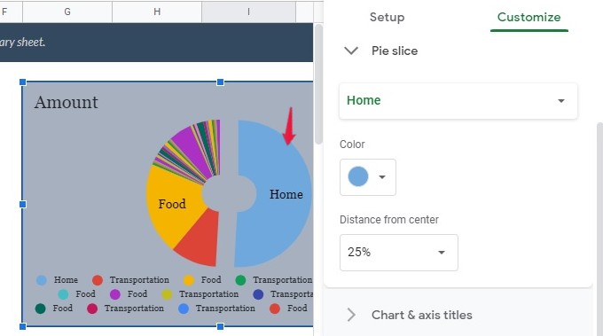
You can change the color of every Pie slice and its distance from the center using the respective drop-down boxes. In this example, the color of the slice titled Home has been changed. Likewise, you can change the color of all Pie slices.

Related: 5 Best Design Collaboration Tools for UI/UX Designers

How to Save/Download Pie Chart from Google Sheets

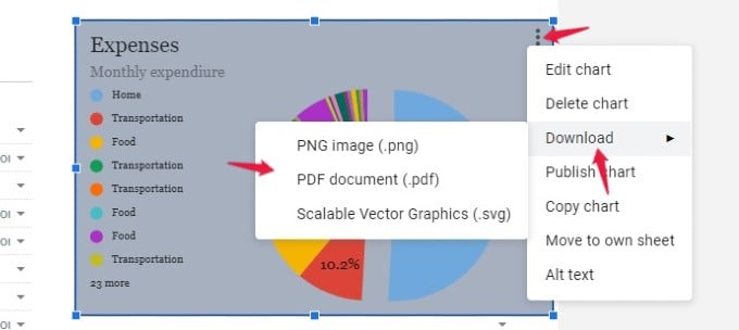
Google Sheet has a cool option to download and save your Pie chart in multiple file formats like .pdf, .png, and .svg. To do that, select the Pie chart and click the three-dot icon on the top right. From the list of options, scroll the mouse over Download and select the desired format.

That’s it. Now, the Pie chart has been successfully saved in your computer in the selected file format.

How to Delete Pie Chart in Google Sheets

Deleting the Pie chart is not a big deal in Google Sheets. Select the Pie chart and press Delete on your keyboard. Or tap the three-dot icon after selecting the Pie chart. Then, click Delete chart. The Pie chart will no longer be displayed on the Google Sheet.

Pie charts will come in handy especially if you are making a presentation to your boss or others during meetings. With the above methods, you can easily make and customize any kind of pie chart and donut chart in Google Sheets.